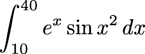
The package consists of the files
   GLOBAL FUNCTION INTEGRATE(function f(x: interval): interval;
                             function fb(xx : interval):b_interval;
                             function fa(xx : interval; r:real):analyticd;
		             a,b, eps:real): interval;


   GLOBAL FUNCTION INTEGRATE(function f(x: interval): interval;
                             function fb(xx : interval):b_interval;
                             function fa(xx : interval; r:real):analyticd;
		             a,b, eps,except:real): interval;

   GLOBAL FUNCTION INTEGRATE(function f(x: interval): interval;
                             function fb(xx : interval):b_interval;
                             function fa(xx : interval; r:real):analyticd;
		             a,b, eps; n:integer): interval;

   GLOBAL FUNCTION INTEGRATE(function f(x: interval): interval;
                             function fb(xx : interval):b_interval;
                             function fa(xx : interval; r:real):analyticd;
		             a,b, eps,except:real; n:integer): interval;
where
As an example and in order to understand the meaning of the parameters, consider the relevant program text from test1.p
   program test (input, output);
   use cinte;
Now, you can use the integration routines
   ....

   function fa1(xx : interval; r:real):analyticd;
   var x : analyticd;
   begin
      x := construct(xx, r);
      fa1:= sin(sqr(x))*exp(x);
   end;

   function fb1(xx : interval):b_interval;
   var x : b_interval;
   begin
      x := construct(xx);
      fb1:= sin(sqr(x))*exp(x);
   end;

   function f1(x : interval): interval;
   begin
      f1 := sin(sqr(x))*exp(x);
   end;
....
In this faster version, the user is required to provide functions for
different types of arguments.
begin
....
    init_cinte;  { preparation for integration - reads all coefficients }
                 { of the used Gaussian quadrature formulas               }
....
( it is faster to read them only once if the integration routine is
called more than once )
....
        integral:= integrate(f1,fb1,fa1, 10.0, 40.0, 1.0e-12);
....
calculates the integral

with an error (see the description of eps above) <1.0e-12
There are two main differences:
   program test (input, output);
   use cinte_comf;

   ....

   function f1(x : inte_type): inte_type;
   begin
      f1 := sin(sqr(x))*exp(x);
   end;
....

begin
   cinte_init;
....

        integral:= integrate(f1, 10.0, 40.0, 1.0e-12);
....
global type b_interval = global record
 int : interval;
   b : boolean;
end;
is defined and an arithmetic is programmed. It is essentially interval arithmetic but the boolean value controls the boundedness. Suppose an operation has to be applied to a b_interval. If b=1 (the initial value), we check if the next operation may yield a floating point exception. If there will be no floating point exception, the operation is applied to the interval and b=1 is kept. Otherwise, the interval is set to [0,0] and the boolean to 0. If b=0, we return the input value.
In order to calculate a bound for the function in a complex neighborhood of an interval, we use the module ade_ari. In this module, the type
global type analyticd = global record
rint, dint : interval;
cint	   : icom;
   a, d	   : boolean;
end;
is defined. rint and dint are bounds for the values and first derivatives respectively. cint is a complex interval. The boolean variables a,d control analyticity of a function/operation on cint and differentiability on rint. Derivatives are calculated with Automatic Differentiation.
The type analyticd contains a component of type icom This represents a complex (rectangular) interval that is symmetric with respect to the real axis:
global type icom =  global record
		re	 : interval;
		im	 : real;
end;
It is particular designed for real problems, i.e., with problems that deal with functions that are analytic as well as real-valued for real arguments. The corresponding arithmetic is faster than arithmetic for the type cinterval
global type inte_type analyticd = global record
rint, dint : interval;
cint	   : icom;
   a, d	   : boolean;
end;
(which is essentially the same as analyticd) serves as a container for interval (only rint is used), for b_interval (only rint and a are used analogously to the components int and b in b_interval) and for analyticd. Switch between the three types represented by inte_type is done in cinte_comf.p by the global variable type_switch (1=interval-operations, 2=b_interval-operations, 3=analyticd-operations)